contour_normal_vectors.py

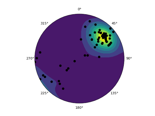
Illustrates plotting normal vectors in “world” coordinates as orientations on a stereonet.

import numpy as np
import matplotlib.pyplot as plt
import mplstereonet

# Load in a series of normal vectors from a triangulated normal fault surface
normals = np.loadtxt('normal_vectors.txt')
x, y, z = normals.T

# Convert these to plunge/bearings for plotting.
# Alternately, we could use xyz2stereonet (it doesn't correct for bi-directional
# measurements, however) or vector2pole.
plunge, bearing = mplstereonet.vector2plunge_bearing(x, y, z)

# Set up the figure
fig = plt.figure()
ax = fig.add_subplot(111, projection='stereonet')

# Make a density contour plot of the orientations
ax.density_contourf(plunge, bearing, measurement='lines')

# Plot the vectors as points on the stereonet.
ax.line(plunge, bearing, marker='o', color='black')

plt.show()

Result