contour_angelier_data.py

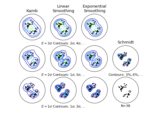
Reproduce Figure 5 from Vollmer, 1995 to illustrate different density contouring methods.

import matplotlib.pyplot as plt
import mplstereonet

import parse_angelier_data

def plot(ax, strike, dip, rake, **kwargs):
    ax.rake(strike, dip, rake, 'ko', markersize=2)
    ax.density_contour(strike, dip, rake, measurement='rakes', linewidths=1,
                       cmap='jet', **kwargs)


# Load data from Angelier, 1979
strike, dip, rake = parse_angelier_data.load()

# Setup a subplot grid
fig, axes = mplstereonet.subplots(nrows=3, ncols=4)

# Hide azimuth tick labels
for ax in axes.flat:
    ax.set_azimuth_ticks([])

contours = [range(2, 18, 2), range(1, 21, 2), range(1, 22, 2)]

# "Standard" Kamb contouring with different confidence levels.
for sigma, ax, contour in zip([3, 2, 1], axes[:, 0], contours):
    # We're reducing the gridsize to more closely match a traditional
    # hand-contouring grid, similar to Kamb's original work and Vollmer's
    # Figure 5. `gridsize=10` produces a 10x10 grid of density estimates.
    plot(ax, strike, dip, rake, method='kamb', sigma=sigma,
        levels=contour, gridsize=10)

# Kamb contouring with inverse-linear smoothing (after Vollmer, 1995)
for sigma, ax, contour in zip([3, 2, 1], axes[:, 1], contours):
    plot(ax, strike, dip, rake, method='linear_kamb', sigma=sigma,
        levels=contour)
    template = r'$E={}\sigma$ Contours: ${}\sigma,{}\sigma,\ldots$'
    ax.set_xlabel(template.format(sigma, *contour[:2]))

# Kamb contouring with exponential smoothing (after Vollmer, 1995)
for sigma, ax, contour in zip([3, 2, 1], axes[:, 2], contours):
    plot(ax, strike, dip, rake, method='exponential_kamb', sigma=sigma,
        levels=contour)

# Title the different methods
methods = ['Kamb', 'Linear\nSmoothing', 'Exponential\nSmoothing']
for ax, title in zip(axes[0, :], methods):
    ax.set_title(title)

# Hide top-right axis... (Need to implement Diggle & Fisher's method)
axes[0, -1].set_visible(False)

# Schmidt contouring (a.k.a. 1%)
plot(axes[1, -1], strike, dip, rake, method='schmidt', gridsize=25,
     levels=range(3, 20, 3))
axes[1, -1].set_title('Schmidt')
axes[1, -1].set_xlabel(r'Contours: $3\%,6\%,\ldots$')

# Raw data.
axes[-1, -1].set_azimuth_ticks([])
axes[-1, -1].rake(strike, dip, rake, 'ko', markersize=2)
axes[-1, -1].set_xlabel('N={}'.format(len(strike)))

plt.show()

Result