kmeans_example.py

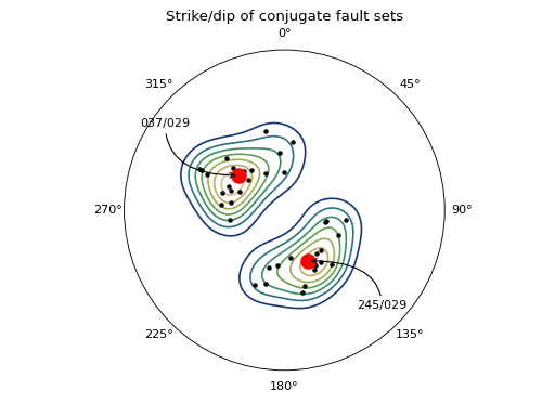
Illustrates finding the average strike and dip of two conjugate sets of faults.

This uses a kmeans approach modified to work with bidirectional orientation measurements in 3D (mplstereonet.kmeans).

import matplotlib.pyplot as plt
import mplstereonet

import parse_angelier_data

# Load data from Angelier, 1979
strike, dip, rake = parse_angelier_data.load()

# Plot the raw data and contour it:
fig, ax = mplstereonet.subplots()
#ax.density_contourf(strike, dip, rake, measurement='rakes', cmap='gist_earth',
#                    sigma=1.5)
ax.density_contour(strike, dip, rake, measurement='rakes', cmap='gist_earth',
                    sigma=1.5)
ax.rake(strike, dip, rake, marker='.', color='black')

# Find the two modes
centers = mplstereonet.kmeans(strike, dip, rake, num=2, measurement='rakes')
strike_cent, dip_cent = mplstereonet.geographic2pole(*zip(*centers))
ax.pole(strike_cent, dip_cent, 'ro', ms=12)

# Label the modes
for (x0, y0) in centers:
    s, d = mplstereonet.geographic2pole(x0, y0)
    x, y = mplstereonet.pole(s, d) # Otherwise, we may get the antipode...

    if x > 0:
        kwargs = dict(xytext=(40, -40), ha='left')
    else:
        kwargs = dict(xytext=(-40, 40), ha='right')

    ax.annotate('{:03.0f}/{:03.0f}'.format(s[0], d[0]), xy=(x, y),
                xycoords='data', textcoords='offset points',
                arrowprops=dict(arrowstyle='->', connectionstyle='angle3'),
                **kwargs)

ax.set_title('Strike/dip of conjugate fault sets', y=1.07)

plt.show()

Result