fisher_stats.py

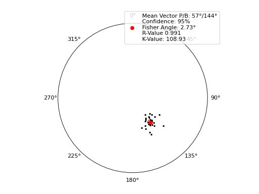
This example shows how the Fisher statistics can be computed and displayed.

Based on example 5.21 and example 5.23 in [Fisher1993].

Data in:	Table B2	(page 279)
Mean Vector:	144.2/57.2	(page 130)
K-Value:	109	(page 130)
Fisher-Angle:	2.7 deg.	(page 132)

Reference

[Fisher1993]

Fisher, N.I., Lewis, T., Embleton, B.J.J. (1993) “Statistical Analysis of Spherical Data”

import matplotlib.pyplot as plt
import mplstereonet as mpl


decl = [122.5, 130.5, 132.5, 148.5, 140.0, 133.0, 157.5, 153.0, 140.0, 147.5,
        142.0, 163.5, 141.0, 156.0, 139.5, 153.5, 151.5, 147.5, 141.0, 143.5,
        131.5, 147.5, 147.0, 149.0, 144.0, 139.5]
incl = [55.5, 58.0, 44.0, 56.0, 63.0, 64.5, 53.0, 44.5, 61.5, 54.5, 51.0, 56.0,
        59.5, 56.5, 54.0, 47.5, 61.0, 58.5, 57.0, 67.5, 62.5, 63.5, 55.5, 62.0,
        53.5, 58.0]
confidence = 95

fig = plt.figure()
ax = fig.add_subplot(111, projection='stereonet')
ax.line(incl, decl, color="black", markersize=2)

vector, stats = mpl.find_fisher_stats(incl, decl, conf=confidence)

template = (u"Mean Vector P/B: {plunge:0.0f}\u00B0/{bearing:0.0f}\u00B0\n"
            "Confidence: {conf}%\n"
            u"Fisher Angle: {fisher:0.2f}\u00B0\n"
            u"R-Value {r:0.3f}\n"
            "K-Value: {k:0.2f}")

label = template.format(plunge=vector[0], bearing=vector[1], conf=confidence,
                        r=stats[0], fisher=stats[1], k=stats[2])

ax.line(vector[0], vector[1], color="red", label=label)
ax.cone(vector[0], vector[1], stats[1], facecolor="None", edgecolor="red")

ax.legend(bbox_to_anchor=(1.1, 1.1), numpoints=1)
plt.show()

Result